DataManyo

Relief-F는 데이터 마이닝 및 머신러닝에서 특징 선택을 위해 사용되는 알고리즘입니다. Relief 알고리즘의 확장판으로, 멀티 클래스 문제를 처리할 수 있고, 불완전하거나 잡음이 많은 데이터에 대한 강건성을 향상시킵니다. 

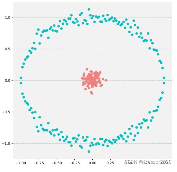
Relief-F 알고리즘의 주요 아이디어는 원래 클래스와 가장 가까운 인스턴스(이웃)와 가장 가까운 인스턴스 중 다른 클래스를 각각 찾는 것입니다. 이를 통해 각 특징이 클래스 구분에 얼마나 중요한지 평가하고, 중요도에 따라 특징을 선택합니다.

Relief-F 알고리즘의 기본적인 단계는 다음과 같습니다:

1. 각 특징의 가중치를 0으로 초기화합니다.
2. 지정된 횟수만큼 다음 과정을 반복합니다:
    - 무작위로 인스턴스를 선택합니다.
    - 선택한 인스턴스와 같은 클래스의 가장 가까운 이웃을 찾습니다.
    - 선택한 인스턴스와 다른 클래스의 가장 가까운 이웃을 찾습니다.
    - 각 특징에 대해, 선택한 인스턴스와 같은 클래스의 이웃과의 차이를 계산하고 가중치에서 빼줍니다.
    - 각 특징에 대해, 선택한 인스턴스와 다른 클래스의 이웃과의 차이를 계산하고 가중치에 더해줍니다.
3. 모든 특징의 가중치를 확인하고, 가중치가 높은 특징부터 낮은 특징까지 순서대로 나열합니다.

위의 방법을 통해 Relief-F 알고리즘은 특징 선택을 위한 중요도 순서를 제공하게 됩니다. 이 알고리즘은 특히 특징 간의 상호작용이 예측 성능에 영향을 미치는 경우 유용합니다.

Relief 알고리즘을 직접 코드로 구현하는 것은 조금 복잡할 수 있지만, 이해를 돕기 위해 기본적인 아이디어를 파이썬 코드로 표현해 보겠습니다.

다음 코드는 실제 Relief 알고리즘의 간략화 된 버전이며, 실제로 작동하려면 입력 데이터와 함께 조정 및 추가 구현이 필요합니다.

또한, 이 코드는 scikit-learn 라이브러리의 K-Nearest Neighbors(KNN) 알고리즘을 사용하여 가장 가까운 이웃을 찾습니다.

import numpy as np
from sklearn.neighbors import NearestNeighbors

def relief(X, y, m):
    """
    X : Data instances
    y : Class labels
    m : Number of sampled instances
    """

    # Initialize a weight vector to zeros
    weights = np.zeros(X.shape[1])
    for i in range(m):
        # Randomly select an instance
        idx = np.random.randint(0, X.shape[0])

        # Split the data into same and different class
        same_class = X[y==y[idx]]
        diff_class = X[y!=y[idx]]

        # Find the nearest neighbor from the same class
        nn_same = NearestNeighbors(n_neighbors=1).fit(same_class)
        distances_same, indices_same = nn_same.kneighbors(X[idx].reshape(1, -1))
        near_same = same_class[indices_same[0][0]]

        # Find the nearest neighbor from the different class
        nn_diff = NearestNeighbors(n_neighbors=1).fit(diff_class)
        distances_diff, indices_diff = nn_diff.kneighbors(X[idx].reshape(1, -1))
        near_diff = diff_class[indices_diff[0][0]]

        # Update the weights
        weights -= np.square(X[idx] - near_same)
        weights += np.square(X[idx] - near_diff)

    return weights

위의 코드는 Relief 알고리즘의 간략화 된 버전이기 때문에, 실제 데이터세트에 적용하려면 추가적인 사전 처리 단계와 최적화가 필요할 수 있습니다. 예를 들어, 코드는 현재 수치형 속성에만 적용됩니다. 범주형 속성이 있는 경우, 해당 속성을 적절하게 처리해야 할 것입니다. 또한, 거리 메트릭에 따라 결과가 크게 달라질 수 있으므로, 문제에 가장 적합한 메트릭을 선택하는 것이 중요합니다.

DBSCAN의 기본 정의에 기반해, x가 핵심 대상이라면 x 밀도에 의해 커버되는 모든 샘플로 구성된 집합을 X라 한다. X는 연속성(식 9.39)과 최대성(식 9.40)을 만족한다는 사실을 증명하라.

문제 정의에 의해 최대성은 만족.

연속성 만족 증명:

x_i를 핵심 대상이라고 가정한다면, x_j는 x_i밀도에 의해 density-reachable이다. 따라서 핵심 대상 x_k가 존재하고, 이는 x_i와 x_k에 direct density reachable이고, x_k와 x_j 의 direct density reachable이다.

x_k는 핵심 대상이기 때문에 x_k와 x_i는 direct density reachable이다. 

또한 direct density reachable 은 density reachable의 부분집합이기 때문에,

x_k와 x_j는 density reachable이다. 그리고 x_k와 xi는 density reachable이고 x_i와 x_j는 density connected 관계이다.

참고:

• Direct density reachable : 점 p가 점 q의 반경에 들어오고, 점 q가 코어점일 때, "점 p가 점 q로부터 직접적으로 밀도(기반)-도달가능한 관계에 있다"고 한다. 반대의 경우는 성립하지 않음.

• Density reachable : 점 p와 점 q 사이에 p1,p2,⋯,pn,p1=q,pn=pp1,p2,⋯,pn,p1=q,pn=p 들이 있고, 점 pi+1pi+1이 점 pipi로 부터 직접적으로 밀도(기반)-도달가능하다면, "점 p는 점 q로부터 밀도(기반)-도달가능한 관계에 있다."고 한다. 

• Density connected : 만약 두 점 p와 q가 모두 어떤 점 O로 부터 반경 내 MinPts 조건 하에 밀도(기반)-도달가능(density-reachable)하다면 "점 p는 점 q와 반경 내 MinPts 조건 하에 밀도(기반)-연결되었다."고 합니다.
  => (다르게 말하면, p가 O의 친구이고, q도 O의 친구이면, p와 q는 친구 O를 통해 서로 연결되었다고 보면 된다.)

설명 출처:

https://syj9700.tistory.com/40#:~:text=Direct%20density%20reachable%20%3A%20%EC%A0%90%20p,%EA%B4%80%EA%B3%84%EC%97%90%20%EC%9E%88%EB%8B%A4%22%EA%B3%A0%20%ED%95%9C%EB%8B%A4.

참고 코드:

import numpy as np
import matplotlib.pyplot as plt
from scipy.spatial import ConvexHull


class KMeans(object):

    def __init__(self, k):
        self.k = k

    def fit(self, X, initial_centroid_index=None, max_iters=10, seed=16, plt_process=False):
        m, n = X.shape

        # 특별히 지정한 중심점이 없으면, 중심점을 랜덤으로 초기화
        if initial_centroid_index is None:
            np.random.seed(seed)
            initial_centroid_index = np.random.randint(0, m, self.k)

        centroid = X[initial_centroid_index, :]

        idx = None

        
        plt.ion()
        for i in range(max_iters):
            # 중심점을 기점으로 샘플을 분류
            idx = self.find_closest_centroids(X, centroid)

            if plt_process:
                self.plot_converge(X, idx, initial_centroid_index)

            # 중심점 다시 계산
            centroid = self.compute_centroids(X, idx)

        
        plt.ioff()
        plt.show()

        return centroid, idx

    def find_closest_centroids(self, X, centroid):

        
        distance = np.sum((X[:, np.newaxis, :] - centroid) ** 2, axis=2)
        idx = distance.argmin(axis=1)
        return idx

    def compute_centroids(self, X, idx):
        centroids = np.zeros((self.k, X.shape[1]))

        for i in range(self.k):
            centroids[i, :] = np.mean(X[idx == i], axis=0)

        return centroids

    def plot_converge(self, X, idx, initial_idx):
        plt.cla()  

        plt.title("k-meas converge process")
        plt.xlabel('density')
        plt.ylabel('sugar content')

        plt.scatter(X[:, 0], X[:, 1], c='lightcoral')
        
        plt.scatter(X[initial_idx, 0], X[initial_idx, 1], label='initial center', c='k')

       
        for i in range(self.k):
            X_i = X[idx == i]

           
            hull = ConvexHull(X_i).vertices.tolist()
            hull.append(hull[0])
            plt.plot(X_i[hull, 0], X_i[hull, 1], 'c--')

        plt.legend()
        plt.pause(0.5)


if __name__ == '__main__':

    data = np.loadtxt('..\data\watermelon4_0_Ch.txt', delimiter=', ')
    centroid, idx = KMeans(3).fit(data, plt_process=True, seed=24)

참고 답안:

찾을 수 없다. 

K평균 값은 NP하드 문제이다. 또한 식9.24는 non-convex 임.

국부 최적해(local optima)함정에 빠질 수 있다는 것이 k평균군집의 단점.

따라서 k평균 군집을 사용할 때는 중심점 랜덤 초기화를 많이 해주고 최적의 결과를 선택하는 것이 좋음.

거리 척도의 4가지 기본 성질을 먼저 살펴보자.

비음수성(Non-Negativity): 

이기 때문에,

이다.

대칭성:

통일성: 

위 예제처럼 너무 명확해서 생략...

삼각부등식 성질:

표현식이 추상적이라 일반화해서 해를 구하기 힘듬. 간단한 특수 상황 (ex. 집합이 연속 공간일때 평면상에 원을 그려 표현)을 통해 설명하는 것이 좋을듯.

10.1 k최근접 분류기의 코드를 작성하고, 수박 데이터 세트 3.0𝛼상에서 그들의 분류 경계와 의사결정 트리 분류 경계의 차이를 비교해 보아라.

#!/usr/bin/python
# -*- coding:utf-8 -*-
import numpy as np
import matplotlib.pyplot as plt

from sklearn.ensemble import BaggingClassifier
from sklearn.tree import DecisionTreeClassifier

file1 = open('c:\quant\watermelon.csv','r')
data = [line.strip('\n').split(',') for line in file1]
data = np.array(data)
#X = [[float(raw[-7]),float(raw[-6]),float(raw[-5]),float(raw[-4]),float(raw[-3]), float(raw[-2])] for raw in data[1:,1:-1]]

X = [[float(raw[-3]), float(raw[-2])] for raw in data[1:]]
y = [1 if raw[-1]=='1' else 0 for raw in data[1:]]
X = np.array(X)
y = np.array(y)

print(__doc__)

import numpy as np
import matplotlib.pyplot as plt
from matplotlib.colors import ListedColormap
from sklearn import neighbors, datasets

n_neighbors = 5

# import some data to play with
iris = datasets.load_iris()
#X = iris.data[:, :2]  # we only take the first two features. We could
                      # avoid this ugly slicing by using a two-dim dataset
#y = iris.target

h = .02  # step size in the mesh

# Create color maps
cmap_light = ListedColormap(['#FFAAAA', '#AAFFAA', '#AAAAFF'])
cmap_bold = ListedColormap(['#FF0000', '#00FF00', '#0000FF'])

for weights in ['uniform', 'distance']:
    # we create an instance of Neighbours Classifier and fit the data.
    clf = neighbors.KNeighborsClassifier(n_neighbors, weights=weights)
    clf.fit(X, y)

    # Plot the decision boundary. For that, we will assign a color to each
    # point in the mesh [x_min, m_max]x[y_min, y_max].
    x_min, x_max = X[:, 0].min() - 1, X[:, 0].max() + 1
    y_min, y_max = X[:, 1].min() - 1, X[:, 1].max() + 1
    xx, yy = np.meshgrid(np.arange(x_min, x_max, h),
                         np.arange(y_min, y_max, h))
    Z = clf.predict(np.c_[xx.ravel(), yy.ravel()])

    # Put the result into a color plot
    Z = Z.reshape(xx.shape)
    plt.figure()
    plt.pcolormesh(xx, yy, Z, cmap=cmap_light)

    # Plot also the training points
    plt.scatter(X[:, 0], X[:, 1], c=y, cmap=cmap_bold)
    plt.xlim(xx.min(), xx.max())
    plt.ylim(yy.min(), yy.max())
    plt.title("3-Class classification (k = %i, weights = '%s')"
              % (n_neighbors, weights))

plt.show()


출처:https://blog.csdn.net/icefire_tyh/article/details/52243773

참조:

6.6 SVM이 노이즈에 대해 민감한 이유를 설명하라.

참고 답안:

SVM 모델의 결정 경계는 소량의 서포트벡터에만 의존한다. 만약 노이즈가 생기면 서포트벡터 자체에 영향을 미치기 때문에 최종 모형이 변할 수 있다. 

이 때문에 소프트 마진, 하드 마진 개념이 나온 것이다. 

SVM은 이상치에도 민감하지만 scale에도 민감하다.

6.5 가우스 SVM과 RBF 신경망 사이의 관계에 대해 기술하라

RBF신경망에서 은닉층 뉴런 개수를 훈련 데이터 수로 설정하고, 각 샘플을 뉴런 센터(c)로 설정하면, 이때 RBF의 예측 함수는 SVM의 활성화 함수와 동일하다.

두 모델의 차이는 큰 편이라 생각하는데,

- RBF활성화 함수에서 분산을 컨트롤하는 파리미터인 β는 모델에 의해 학습되지만, SVM에서는 하나의 하이퍼파리미터이다.

- 목적함수나 최적화 방식이 다르다

그러나 RBF에서  β를 SVM과 동일하게 고정한다면 훈련 결과는 비슷할 것이다 (추측...)